Introduction

Both Raytracer and Rasterizer are build in Visual Studio using C++ with the OpenGL mathematics (GLM) library and SDL2. The first step for both of them was to render correctly the famous Cornell Box and afterwards there are some extra additions for each method.

Raytracer

Raytracing is a method which draws images of 3D scenes by tracing the light rays reaching the simulated camera.

• The first step is to realise how to represent objects as triangles and triangles as 3 vertices with a normal and a colour. This is a core concept of how items are stored and represented which is not only related to Raytracing but in many major 3D software the idea of how objects are stored is similarly. (Although the representation with only vertices, normal and colour is overly simplistic)
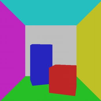
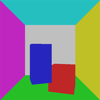
• The core concept of Raytracing is how light bounces around in space. Raytracing is an attempt at simulating that behavior. This is done by shooting rays from the camera towards the objects in the scene and calculating the intersection of that ray with the objects, specifically the closest intersection. By sending a ray from each pixel of the screen through the virtual camera you can get the colour value of the closest intersection for each ray which results in the image shown in Figure 1.

  

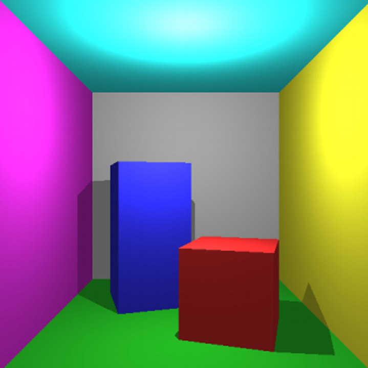
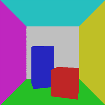
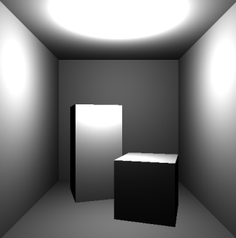
• Direct Illumination: The core step of calculating the intersection of the rays results in an image where the objects have exactly the same colour everywhere without any depth and the feeling of 3D is not present in the image. For more realism light is added, specifically an omni light which spreads light equally in all directions from a single point in space. The light is represented by its position, and its power in each color component. If a surface is further away from the light source it receives less light. Calculating just one "bounce" of light in the scene and not considering colour produces the image shown in Figure 2.

  

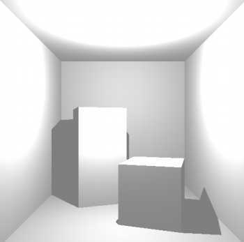
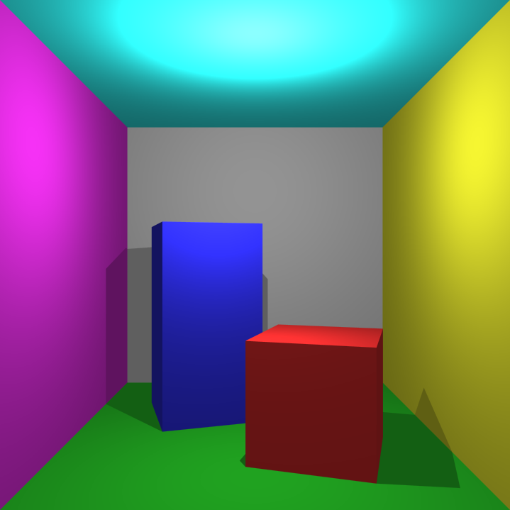
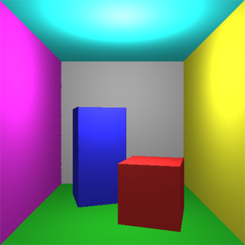
• Indirect Illumination: Just calculating direct illumination makes the image have very dark spots at some points which is not realistic. In the real world some light is absorbed by the material but some of it is reflected. To simplify indirect illumination we assume that all objects in the scene are made of the same material and therefore reflect the same amount of light. The resulting light intensity is shown in Figure 3.

  

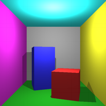
• Direct Shadows: Figure 3 also shows the effects of direct shadows, meaning that if another surface intersects the ray from the light source to the current surface then that surface does not receive direct illumination. This produces a simple sharp shadow. Figure 4 shows the end result when you mix the colours of the surfaces with direct illumination, direct shadows and indirect illumination.

  

• Anti Aliasing: At the edges of the objects there are some visible jagged lines which make the image look low resolution or pixelated, they are especially visible on the red cube. This effect is caused because we draw pixel by pixel without transitioning from object to object making the pixels either the colour of the cube or the colour of the background for example. Anti-aliasing is a method for resolving that problem. In Raytracing anti-aliasing works by using multiple rays for each pixel instead of one and averaging their resulting values. A simple explanation for it is trying to render a higher resolution image and downsizing it. Figure 5 and 6 show the difference between the image without anti-aliasing and the image with level 4 (16 rays for each pixel) anti-aliasing.

  

  

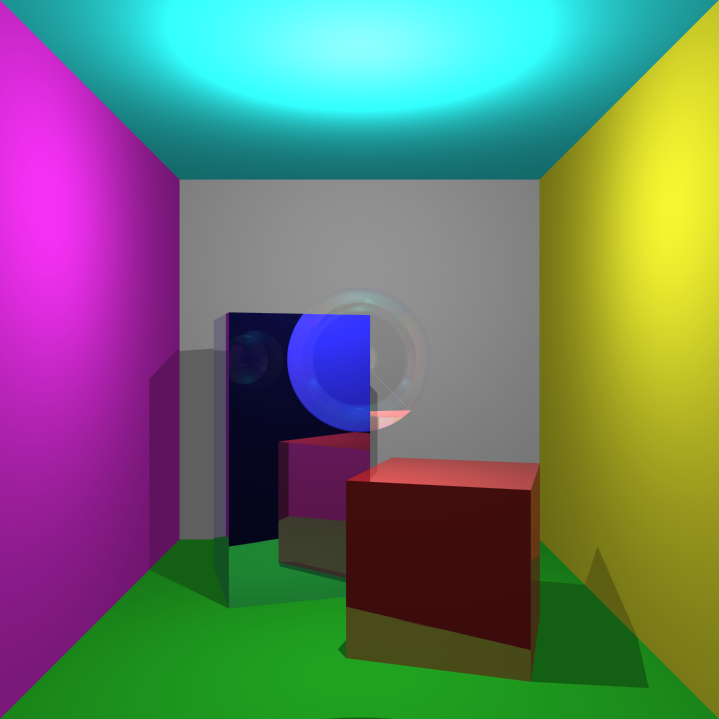
• Experimenting further with the Raytracer, I implemented Reflection, Refraction and combined them through the Fresnel Equation for transparent objects. Raytracing is a very good simulation of the real world which produces realistic and amazing results for computer graphics. It is computationally expensive though and even though optimizations such as Cramer's rule, render even this simple scene with anti-aliasing and reflection/refraction and transparency is very intense for a computer.

  

Rasterizer

Although Raytracing is simple and can simulate all kinds of phenomena, its speed is its disadvantage and therefore it is typically not used for real-time visualization. For those scenarios another method is used called Rasterization. Rasterization is usually faster than Raytracing but it cannot easily and effectively simulate all illumination phenomena.

• The first steps are the same as Raytracing, you have to represent objects using triangles, vertices and edges.
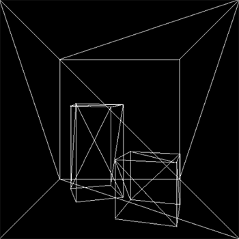
• The concept of Rasterization is to get a 3D image convert it into a series of pixels dots or lines which when displayed together, create the view of the image with shapes. Basically getting a single perspective of the 3D image making it into 2D as a flat picture and then drawing on top correctly to give the illusion of depth. By calculating the projection of the 3 dimensional vertices onto a 2 dimensional plane that we want to view (our screen) we can plot the points and join them to create a wireframe of the image as shown in Figure 8.

  

• Interpolation: In Rasterization interpolating between two points to find the pixels necessary to draw the image is very crucial. To draw inside a triangle correctly, first you need to interpolate between the vertices and find the bounding left and right pixels for each y-level, then you fill the triangle by drawing lines for each y-level reaching between the left the right most pixel at that row. The process is to identify the outline of the triangle and then row by row draw the required colour. Figure 9 shows the result of that process.

  

• Depth Buffer: There is an apparent problem with the image in Figure 9, the blue box is drawn on top of the red box when it should be the opposite. This issue is emerged because the triangles are drawn in order without any consideration for the depth of each triangle and therefore they overwrite the pixel colour. The solution for this issue is to introduce a depth buffer where each pixel drawn on screen keeps some information about its depth and then if another triangle tries to draw on that pixel it will first check if it is in front of the previously drawn pixel and only then it will overwrite it. However the information stored for depth (z value) is not depth it self, its the inverse of depth (1/z value). The reason for storing the inverse of depth is because in 3D the depth is linearly interpolated across two vertices but in its projection in 2D, depth cannot be linearly interpolated, instead the inverse of depth will vary linearly and therefore it makes the interpolating calculations much easier. Figure 10 shows the results after introducing the depth buffer.

  

• Per Pixel illumination: to produce illumination results for each pixel, you have to store the 3D position for every pixel through interpolation and then use that 3D position to calculate the correct colour to be drawn for that pixel. The perspective correct interpolated 3D values need to be calculated otherwise the lighting on the image will look odd. Figure 11 shows the effects of the per pixel illumination.

  

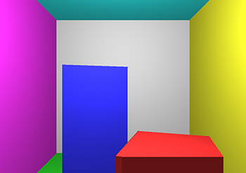
• Clipping: Referencing back to the depth buffer, we said that the inverse of the depth is stored in there but what happens if the depth is 0? Division by zero is a problem and in fact the closer a triangle is to the camera th bigger a number is thus making the division and the storage of the inverse of depth a performance issue. Other issues is that even if objects are behind or not located in the field of view of the screen, are processed. Clipping is a major performance optimization which allows for objects only found in the view space of the camera to be visible which is the left,right, top and bottom clipping but also front and back clipping allows for things that are pretty far away to not be rendered or items behind the camera. Figure 12 shows front clipping where the red box is sliced because it is too close to the camera. Clipping in this example slices the red box and more smaller triangles are created to account for the shape change in the picture. Clipping is usually performed in Homogeneous coordinates as it is an easier method to check if a point lies inside or outside the viewing volume.

  

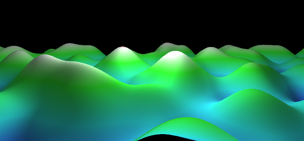
• Procedural Generation and Perlin Noise: Lastly I got involved with some simple procedural generation techniques. I wanted to create a terrain like object that would feel like mountains and valleys, completely generated by a function. Kin Perlin noise is in simple terms a mathematical noise function that when viewed from a distance it seems like the values are randomly generated but when you look at a value you can see that there is a correlation between it and its neighboring values. This property of the function creates a smooth transition between values but also a pseudo-random pattern in general. To create the terrain, I started by generating a flat grid of vertices and then joining them in triangles. Using a 2 dimensional version of the Perlin noise, I determined each vertex height (y-value) from its x and z coordinate and matched it to a point in Perlin noise function. Playing around with the scale of the Perlin noise in order to find a configuration that seemed good. To finish off the "illusion" of a terrain I added a colour pallette so that low height levels would be blue, then cyan, then green then white with a blending option between the colours for a smooth transition. The end result is shown in Figure 13.